The vertical axis represents the value of the Hinge loss (in blue) and zero-one loss (in green) for fixed t = 1, while the horizontal axis represents the value of the prediction y. The plot shows that the Hinge loss penalizes predictions y < 1, corresponding to the notion of a margin in a support vector machine.

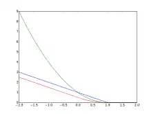
In machine learning, the hinge loss is a loss function used for training classifiers. The hinge loss is used for "maximum-margin" classification, most notably for support vector machines (SVMs).^[1]

For an intended output t = ±1 and a classifier score y, the hinge loss of the prediction y is defined as

${\displaystyle \ell (y)=\max(0,1-t\cdot y)}$

Note that ${\displaystyle y}$ should be the "raw" output of the classifier's decision function, not the predicted class label. For instance, in linear SVMs, ${\displaystyle y=\mathbf {w} \cdot \mathbf {x} +b}$, where ${\displaystyle (\mathbf {w} ,b)}$ are the parameters of the hyperplane and ${\displaystyle \mathbf {x} }$ is the input variable(s).

When t and y have the same sign (meaning y predicts the right class) and ${\displaystyle |y|\geq 1}$, the hinge loss ${\displaystyle \ell (y)=0}$. When they have opposite signs, ${\displaystyle \ell (y)}$ increases linearly with y, and similarly if ${\displaystyle |y|<1}$, even if it has the same sign (correct prediction, but not by enough margin).

Extensions

While binary SVMs are commonly extended to multiclass classification in a one-vs.-all or one-vs.-one fashion,^[2] it is also possible to extend the hinge loss itself for such an end. Several different variations of multiclass hinge loss have been proposed.^[3] For example, Crammer and Singer^[4] defined it for a linear classifier as^[5]

${\displaystyle \ell (y)=\max(0,1+\max _{y\neq t}\mathbf {w} _{y}\mathbf {x} -\mathbf {w} _{t}\mathbf {x} )}$,

where ${\displaystyle t}$ is the target label, ${\displaystyle \mathbf {w} _{t}}$ and ${\displaystyle \mathbf {w} _{y}}$ are the model parameters.

Weston and Watkins provided a similar definition, but with a sum rather than a max:^[6][3]

${\displaystyle \ell (y)=\sum _{y\neq t}\max(0,1+\mathbf {w} _{y}\mathbf {x} -\mathbf {w} _{t}\mathbf {x} )}$.

In structured prediction, the hinge loss can be further extended to structured output spaces. Structured SVMs with margin rescaling use the following variant, where w denotes the SVM's parameters, y the SVM's predictions, φ the joint feature function, and Δ the Hamming loss:

${\displaystyle {\begin{aligned}\ell (\mathbf {y} )&=\max(0,\Delta (\mathbf {y} ,\mathbf {t} )+\langle \mathbf {w} ,\phi (\mathbf {x} ,\mathbf {y} )\rangle -\langle \mathbf {w} ,\phi (\mathbf {x} ,\mathbf {t} )\rangle )\\&=\max(0,\max _{y\in {\mathcal {Y}}}\left(\Delta (\mathbf {y} ,\mathbf {t} )+\langle \mathbf {w} ,\phi (\mathbf {x} ,\mathbf {y} )\rangle \right)-\langle \mathbf {w} ,\phi (\mathbf {x} ,\mathbf {t} )\rangle )\end{aligned}}}$.

Optimization

The hinge loss is a convex function, so many of the usual convex optimizers used in machine learning can work with it. It is not differentiable, but has a subgradient with respect to model parameters w of a linear SVM with score function ${\displaystyle y=\mathbf {w} \cdot \mathbf {x} }$ that is given by

${\displaystyle {\frac {\partial \ell }{\partial w_{i}}}={\begin{cases}-t\cdot x_{i}&{\text{if }}t\cdot y<1,\\0&{\text{otherwise}}.\end{cases}}}$

Plot of three variants of the hinge loss as a function of z = ty: the "ordinary" variant (blue), its square (green), and the piece-wise smooth version by Rennie and Srebro (red). The y-axis is the l(y) hinge loss, and the x-axis is the parameter t

However, since the derivative of the hinge loss at ${\displaystyle ty=1}$ is undefined, smoothed versions may be preferred for optimization, such as Rennie and Srebro's^[7]

${\displaystyle \ell (y)={\begin{cases}{\frac {1}{2}}-ty&{\text{if}}~~ty\leq 0,\\{\frac {1}{2}}(1-ty)^{2}&{\text{if}}~~0<ty<1,\\0&{\text{if}}~~1\leq ty\end{cases}}}$

or the quadratically smoothed

${\displaystyle \ell _{\gamma }(y)={\begin{cases}{\frac {1}{2\gamma }}\max(0,1-ty)^{2}&{\text{if}}~~ty\geq 1-\gamma ,\\1-{\frac {\gamma }{2}}-ty&{\text{otherwise}}\end{cases}}}$

suggested by Zhang.^[8] The modified Huber loss ${\displaystyle L}$ is a special case of this loss function with ${\displaystyle \gamma =2}$, specifically ${\displaystyle L(t,y)=4\ell _{2}(y)}$.

See also

• Multivariate adaptive regression spline § Hinge functions

References

- ↑ Rosasco, L.; De Vito, E. D.; Caponnetto, A.; Piana, M.; Verri, A. (2004). "Are Loss Functions All the Same?" (PDF). Neural Computation. 16 (5): 1063–1076. CiteSeerX 10.1.1.109.6786. doi:10.1162/089976604773135104. PMID 15070510.
- ↑ Duan, K. B.; Keerthi, S. S. (2005). "Which Is the Best Multiclass SVM Method? An Empirical Study" (PDF). Multiple Classifier Systems. LNCS. Vol. 3541. pp. 278–285. CiteSeerX 10.1.1.110.6789. doi:10.1007/11494683_28. ISBN 978-3-540-26306-7.
- 1 2 Doğan, Ürün; Glasmachers, Tobias; Igel, Christian (2016). "A Unified View on Multi-class Support Vector Classification" (PDF). Journal of Machine Learning Research. 17: 1–32.
- ↑ Crammer, Koby; Singer, Yoram (2001). "On the algorithmic implementation of multiclass kernel-based vector machines" (PDF). Journal of Machine Learning Research. 2: 265–292.
- ↑ Moore, Robert C.; DeNero, John (2011). "L1 and L2 regularization for multiclass hinge loss models" (PDF). Proc. Symp. on Machine Learning in Speech and Language Processing.
- ↑ Weston, Jason; Watkins, Chris (1999). "Support Vector Machines for Multi-Class Pattern Recognition" (PDF). European Symposium on Artificial Neural Networks.
- ↑ Rennie, Jason D. M.; Srebro, Nathan (2005). Loss Functions for Preference Levels: Regression with Discrete Ordered Labels (PDF). Proc. IJCAI Multidisciplinary Workshop on Advances in Preference Handling.
- ↑ Zhang, Tong (2004). Solving large scale linear prediction problems using stochastic gradient descent algorithms (PDF). ICML.