The difference between a small and large Gaussian blur

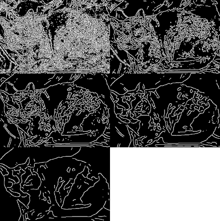
In image processing, a Gaussian blur (also known as Gaussian smoothing) is the result of blurring an image by a Gaussian function (named after mathematician and scientist Carl Friedrich Gauss).

It is a widely used effect in graphics software, typically to reduce image noise and reduce detail. The visual effect of this blurring technique is a smooth blur resembling that of viewing the image through a translucent screen, distinctly different from the bokeh effect produced by an out-of-focus lens or the shadow of an object under usual illumination.

Gaussian smoothing is also used as a pre-processing stage in computer vision algorithms in order to enhance image structures at different scales—see scale space representation and scale space implementation.

Mathematics

Mathematically, applying a Gaussian blur to an image is the same as convolving the image with a Gaussian function. This is also known as a two-dimensional Weierstrass transform. By contrast, convolving by a circle (i.e., a circular box blur) would more accurately reproduce the bokeh effect.

Since the Fourier transform of a Gaussian is another Gaussian, applying a Gaussian blur has the effect of reducing the image's high-frequency components; a Gaussian blur is thus a low-pass filter.

A halftone print rendered smooth through Gaussian blur

The Gaussian blur is a type of image-blurring filter that uses a Gaussian function (which also expresses the normal distribution in statistics) for calculating the transformation to apply to each pixel in the image. The formula of a Gaussian function in one dimension is

$${\displaystyle G(x)={\frac {1}{\sqrt {2\pi \sigma ^{2}}}}e^{-{\frac {x^{2}}{2\sigma ^{2}}}}}$$

In two dimensions, it is the product of two such Gaussian functions, one in each dimension:^[1][2][3]

$${\displaystyle G(x,y)={\frac {1}{2\pi \sigma ^{2}}}e^{-{\frac {x^{2}+y^{2}}{2\sigma ^{2}}}}}$$

where x is the distance from the origin in the horizontal axis, y is the distance from the origin in the vertical axis, and σ is the standard deviation of the Gaussian distribution. It is important to note that the origin on these axes are at the center (0, 0). When applied in two dimensions, this formula produces a surface whose contours are concentric circles with a Gaussian distribution from the center point.

Values from this distribution are used to build a convolution matrix which is applied to the original image. This convolution process is illustrated visually in the figure on the right. Each pixel's new value is set to a weighted average of that pixel's neighborhood. The original pixel's value receives the heaviest weight (having the highest Gaussian value) and neighboring pixels receive smaller weights as their distance to the original pixel increases. This results in a blur that preserves boundaries and edges better than other, more uniform blurring filters; see also scale space implementation.

In theory, the Gaussian function at every point on the image will be non-zero, meaning that the entire image would need to be included in the calculations for each pixel. In practice, when computing a discrete approximation of the Gaussian function, pixels at a distance of more than 3σ have a small enough influence to be considered effectively zero. Thus contributions from pixels outside that range can be ignored. Typically, an image processing program need only calculate a matrix with dimensions ${\displaystyle \lceil 6\sigma \rceil }$ × ${\displaystyle \lceil 6\sigma \rceil }$ (where ${\displaystyle \lceil \cdot \rceil }$ is the ceiling function) to ensure a result sufficiently close to that obtained by the entire Gaussian distribution.

In addition to being circularly symmetric, the Gaussian blur can be applied to a two-dimensional image as two independent one-dimensional calculations, and so is termed a separable filter. That is, the effect of applying the two-dimensional matrix can also be achieved by applying a series of single-dimensional Gaussian matrices in the horizontal direction, then repeating the process in the vertical direction. In computational terms, this is a useful property, since the calculation can be performed in ${\displaystyle O\left(w_{\text{kernel}}w_{\text{image}}h_{\text{image}}\right)+O\left(h_{\text{kernel}}w_{\text{image}}h_{\text{image}}\right)}$ time (where h is height and w is width; see Big O notation), as opposed to ${\displaystyle O\left(w_{\text{kernel}}h_{\text{kernel}}w_{\text{image}}h_{\text{image}}\right)}$ for a non-separable kernel.

Applying successive Gaussian blurs to an image has the same effect as applying a single, larger Gaussian blur, whose radius is the square root of the sum of the squares of the blur radii that were actually applied. For example, applying successive Gaussian blurs with radii of 6 and 8 gives the same results as applying a single Gaussian blur of radius 10, since ${\displaystyle {\sqrt {6^{2}+8^{2}}}=10}$. Because of this relationship, processing time cannot be saved by simulating a Gaussian blur with successive, smaller blurs — the time required will be at least as great as performing the single large blur.

Two downscaled images of the Flag of the Commonwealth of Nations. Before downscaling, a Gaussian blur was applied to the bottom image but not to the top image. The blur makes the image less sharp, but prevents the formation of moiré pattern aliasing artifacts.

Gaussian blurring is commonly used when reducing the size of an image. When downsampling an image, it is common to apply a low-pass filter to the image prior to resampling. This is to ensure that spurious high-frequency information does not appear in the downsampled image (aliasing). Gaussian blurs have nice properties, such as having no sharp edges, and thus do not introduce ringing into the filtered image.

Low-pass filter

Gaussian blur is a low-pass filter, attenuating high frequency signals.^[3]

Its amplitude Bode plot (the log scale in the frequency domain) is a parabola.

Variance reduction

How much does a Gaussian filter with standard deviation ${\displaystyle \sigma _{f}}$ smooth the picture? In other words, how much does it reduce the standard deviation of pixel values in the picture? Assume the grayscale pixel values have a standard deviation ${\displaystyle \sigma _{X}}$, then after applying the filter the reduced standard deviation ${\displaystyle \sigma _{r}}$ can be approximated as

$${\displaystyle \sigma _{r}\approx {\frac {\sigma _{X}}{\sigma _{f}2{\sqrt {\pi }}}}.}$$

Sample Gaussian matrix

This sample matrix is produced by sampling the Gaussian filter kernel (with σ = 0.84089642) at the midpoints of each pixel and then normalizing. The center element (at [0, 0]) has the largest value, decreasing symmetrically as distance from the center increases. Since the filter kernel's origin is at the center, the matrix starts at ${\textstyle G(-R,-R)}$ and ends at ${\textstyle G(R,R)}$ where R equals the kernel radius.

$${\displaystyle {\begin{bmatrix}0.00000067&0.00002292&{\textbf {0.00019117}}&0.00038771&{\textbf {0.00019117}}&0.00002292&0.00000067\\0.00002292&0.00078633&0.00655965&0.01330373&0.00655965&0.00078633&0.00002292\\{\textbf {0.00019117}}&0.00655965&0.05472157&0.11098164&0.05472157&0.00655965&{\textbf {0.00019117}}\\0.00038771&0.01330373&0.11098164&{\textbf {0.22508352}}&0.11098164&0.01330373&0.00038771\\{\textbf {0.00019117}}&0.00655965&0.05472157&0.11098164&0.05472157&0.00655965&{\textbf {0.00019117}}\\0.00002292&0.00078633&0.00655965&0.01330373&0.00655965&0.00078633&0.00002292\\0.00000067&0.00002292&{\textbf {0.00019117}}&0.00038771&{\textbf {0.00019117}}&0.00002292&0.00000067\end{bmatrix}}}$$

The element 0.22508352 (the central one) is 1177 times larger than 0.00019117 which is just outside 3σ.

Implementation

A Gaussian blur effect is typically generated by convolving an image with an FIR kernel of Gaussian values.

In practice, it is best to take advantage of the Gaussian blur’s separable property by dividing the process into two passes. In the first pass, a one-dimensional kernel is used to blur the image in only the horizontal or vertical direction. In the second pass, the same one-dimensional kernel is used to blur in the remaining direction. The resulting effect is the same as convolving with a two-dimensional kernel in a single pass, but requires fewer calculations.

Discretization is typically achieved by sampling the Gaussian filter kernel at discrete points, normally at positions corresponding to the midpoints of each pixel. This reduces the computational cost but, for very small filter kernels, point sampling the Gaussian function with very few samples leads to a large error. In these cases, accuracy is maintained (at a slight computational cost) by integration of the Gaussian function over each pixel's area.^[4]

When converting the Gaussian’s continuous values into the discrete values needed for a kernel, the sum of the values will be different from 1. This will cause a darkening or brightening of the image. To remedy this, the values can be normalized by dividing each term in the kernel by the sum of all terms in the kernel.

A much better and theoretically more well-founded approach is to instead perform the smoothing with the discrete analogue of the Gaussian kernel,^[5] which possesses similar properties over a discrete domain as makes the continuous Gaussian kernel special over a continuous domain, for example, the kernel corresponding to the solution of a diffusion equation describing a spatial smoothing process, obeying a semi-group property over additions of the variance of the kernel, or describing the effect of Brownian motion over a spatial domain, and with the sum of its values being exactly equal to 1. For a more detailed description about the discrete analogue of the Gaussian kernel, see the article on scale-space implementation and.^[5]

The efficiency of FIR breaks down for high sigmas. Alternatives to the FIR filter exist. These include the very fast multiple box blurs, the fast and accurate IIR Deriche edge detector, a "stack blur" based on the box blur, and more.^[6]

Time-causal temporal smoothing

For processing pre-recorded temporal signals or video, the Gaussian kernel can also be used for smoothing over the temporal domain, since the data are pre-recorded and available in all directions. When processing temporal signals or video in real-time situations, the Gaussian kernel cannot, however, be used for temporal smoothing, since it would access data from the future, which obviously cannot be available. For temporal smoothing in real-time situations, one can instead use the temporal kernel referred to as the time-causal limit kernel,^[7] which possesses similar properties in a time-causal situation (non-creation of new structures towards increasing scale and temporal scale covariance) as the Gaussian kernel obeys in the non-causal case. The time-causal limit kernel corresponds to convolution with an infinite number of truncated exponential kernels coupled in cascade, with specifically chosen time constants. For discrete data, this kernel can often be numerically well approximated by a small set of first-order recursive filters coupled in cascade, see ^[7] for further details.

Common uses

This shows how smoothing affects edge detection. With more smoothing, fewer edges are detected

See also

• Difference of Gaussians
• Image noise
• Gaussian filter
• Gaussian pyramid
• Infinite impulse response (IIR)
• Scale space implementation
• Median filter
• Weierstrass transform

Notes and references

External links

• GLSL implementation of a separable gaussian blur filter.
• Example for Gaussian blur (low-pass filtering) applied to a wood-block print and an etching in order to remove details for picture comparison.
• Mathematica GaussianFilter function

• OpenCV (C++) GaussianBlur function